
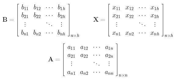
Since solving a system of linear equations is a basic skill that will be used for interpolation and approximation, we will briefly discuss a commonly used technique here. In fact, what we will be using is a slightly more general form. Suppose we have a n×n coefficient matrix A, a n×h "constant" term matrix B, and a n×h unknown matrix X defined as follows:
Suppose further that they satisfy the following relation:
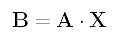
If A and B are known, we need a fast method to solve for X. One may suggest the following: compute the inverse matrix A-1 of A and the solution is simply X = A-1B. While this is a correct way to solve the problem, it is a little overkill. One might also observe the following fact: column j of matrix B is the product of matrix A and column j of matrix X as shown below:
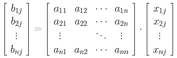
With this in mind, we can solve column j of X using A and column j of B. In this way, the given problem is equivalent to solving h systems of linear equations. Actually, this is not a good strategy either because in solving for column 1 of X matrix A will be destroyed, and, as a result, for each column we need to make a copy of matrix A before running the linear system solver.
So, we need a method that does not use matrix inversion and does not have to copy matrix A over and over. A possible way is the use of the LU decomposition technique.
LU Decomposition
An efficient procedure for solving B = A.X is the LU-decomposition. While other methods such as Gaussian elimination method and Cholesky method can do the job well, this LU-decomposition method can help accelerate the computation.
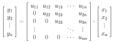
The LU-decomposition method first "decomposes" matrix A into A = L.U, where L and U are lower triangular and upper triangular matrices, respectively. More precisely, if A is a n×n matrix, L and U are also n×n matrices with forms like the following:
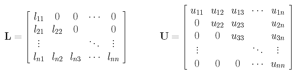
The lower triangular matrix L has zeros in all entries above its diagonal and the upper triangular matrix U has zeros in all entries below its diagonal. If the LU-decomposition of A = L.U is found, the original equation becomes B = (L.U).X. This equation can be rewritten as B = L.(U.X). Since L and B are known, solving for B = L.Y gives Y = U.X. Then, since U and Y are known, solving for X from Y = U.Xyields the desired result. In this way, the original problem of solving for X from B = A.X is decomposed into two steps:
- Solving for Y from B = L.Y
- Solving for X from Y = U.X
Forward Substitution
How easy are these two steps? It turns out to be very easy. Consider the first step. Expanding B = L.Y gives
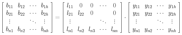
It is not difficult to verify that column j of matrix B is the product of matrix A and column j of matrix Y. Therefore, we can solve one column of Y at a time. This is shown below:
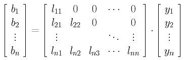
This equation is equivalent to the following:
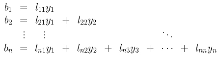
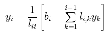
From the above equations, we see that y1 = b1/l11. Once we have y1 available, the second equation yields y2 = (b2-l21y1)/l22. Now we have y1 and y2, from equation 3, we have y3 = (b3 - (l31y1 +l32y2)/l33. Thus, we compute y1 from the first equation and substitute it into the second to compute y2. Once y1 and y2 are available, they are substituted into the third equation to solve for y3. Repeating this process, when we reach equation i, we will have y1, y2, ..., yi-1 available. Then, they are substituted into equation i to solve for yi using the following formula:
Because the values of the yi's are substituted to solve for the next value of y, this process is referred to as forward substitution. We can repeat the forward substitution process for each column of Y and its corresponding column of B. The result is the solution Y. The following is an algorithm:
Input: Matrix Bn×h and a lower triangular matrix Ln×h
Output: Matrix Yn×h such that B = L.Y holds.
Algorithm:/* there are h columns */
for j := 1 to h do/* do the following for each column */
begin/* compute y1 of the current column */
end
y1,j = b1,j / l1,1;
for i := 2 to n do /* process elements on that column */begin
sum := 0; /* solving for yi of the current column */
end
for k := 1 to i-1 dosum := sum + li,k× yk,j;
yi,j = (bi,j - sum)/li,i;
Backward Substitution
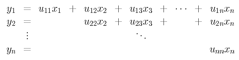
After Y becomes available, we can solve for X from Y = U.X. Expanding this equation and only considering a particular column of Y and the corresponding column of X yields the following:
This equation is equivalent to the following:
Now, xn is immediately available from equation n, because xn = yn/un,n. Once xn is available, plugging it into equation n-1
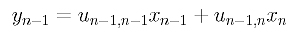
and solving for xn-1 yields xn-1 = (yn-1- un-1,nxn)/ un-1,n-1. Now, we have xn and xn-1. Plugging them into equation n-2

and solving for xn-2 yields xn-2 = [yn-2- (un-2,n-1xn-1 + un-2,nxn-)]/ un-2,n-2.
From xn, xn-1 and xn-2, we can solve for xn-3 from equation n-3. In general, after xn, xn-1, ..., xi+1 become available, we can solve for xi from equation i using the following relation:
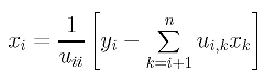
Repeat this process until x1 is computed. Then, all unknown x's are available and the system of linear equations is solved. The following algorithm summarizes this process:
Input: Matrix Yn×h and a upper triangular matrix Un×h
Output: Matrix Xn×h such that Y = U.X holds.
Algorithm:/* there are h columns */
for j := 1 to h do/* do the following for each column */
begin/* compute xn of the current column */
end
xn,j = yn,j / un,n;
for i := n-1 downto 1 do /* process elements of that column */begin
sum := 0; /* solving for xi on the current column */
end
for k := i+1 to n dosum := sum + ui,k× xk,j;
xi,j = (yi,j - sum)/ui,i;
This time we work backward, from xn backward to x1, and, hence, this process is referred to as backward substitution.


0 comments:
Post a Comment